LAB 6
Today’s lab will focus on accessing formatted data using Pandas and Unix shell scripts.
Software tools needed: web browser and Python IDLE programming environment with the Pandas package installed.
In-class Quiz
During lab, there is a quiz. The password to access the quiz will be given during lab. To complete the quiz, log on to Blackboard (see Lab 1 for details on using Blackboard).
Using Python, Gradescope, and Blackboard
See Lab 1 for details on using Python, Gradescope, and Blackboard.
Pandas & Reading Data
To make reading files easier, we will use the Pandas library that lets
you read in structured data files very efficiently.
Pandas, Python Data Analysis Library, is an elegant, open-source package for
extracting, manipulating, and analyzing data, especially those stored in
2D arrays (like spreadsheets). It incorporates most of the Python
constructs and libraries that we have seen thus far.
(Pandas is
installed with anacondaLab 1 for
installing packages for Python.)
In Pandas, the
basic structure is a DataFrame which stored data in rectangular grids.
Let’s use this to visualize the change in New York City’s population.
First, start your file with an import statements for pyplot and pandas:
import matplotlib.pyplot as plt
import pandas as pd
We used matplotlib in the Lab 3 and Lab 4 for plotting. The as plt allows us to use the plotting commands without having to write matplotlib.pyplot everytime, instead we just write plt. Similarly, The as pd allows us to use pandas commands without writing out pandas everytime– we just write pd.
Next, save the NYC historical population data to the same directory as your program. This is a “comma separated values” file– which is a plain text file containging spreadsheet data, with commas separating the different columns (thus, the name). Here’s the first 10 lines of the file:
Source:  https://en.wikipedia.org/wiki/Demographics\_of\_New\_York\_City,,,,,,
\* All population figures are consistent with present-day boundaries.,,,,,,
First census after the consolidation of the five boroughs,,,,,,
,,,,,,
,,,,,,
Year,Manhattan,Brooklyn,Queens,Bronx,Staten Island,Total
1698,4937,2017,,,727,7681
1771,21863,3623,,,2847,28423
1790,33131,4549,6159,1781,3827,49447
1800,60515,5740,6642,1755,4563,79215
Note that it has 5 extra lines at the top before the column names occur. The pandas function for reading in CSV files is read_csv(). It has an option to skip rows which we will use here:
pop = pd.read_csv('nycHistPop.csv',skiprows=5)
Before going on, let’s print out the variable pop. pop is a dataframe, described in the reading above:
print(pop)
The last line of our first pandas program is:
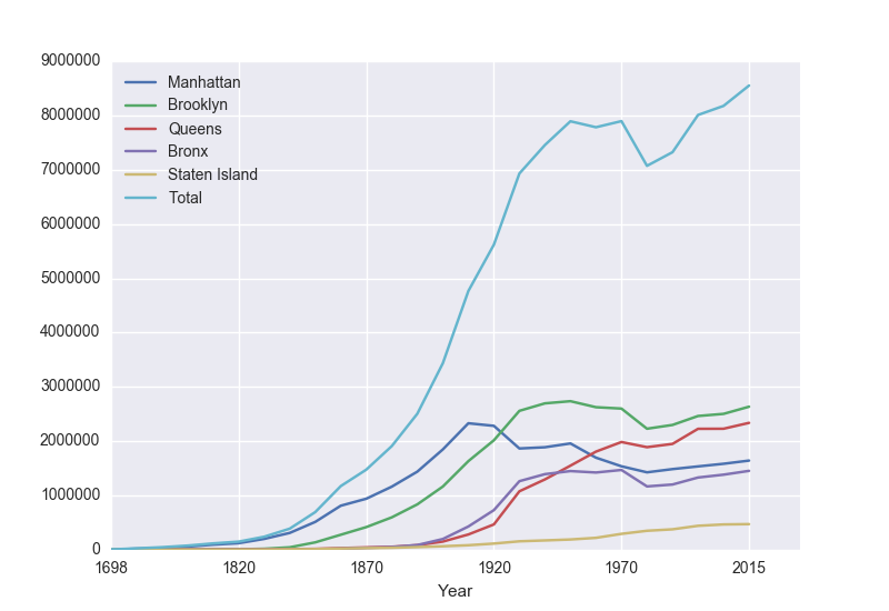
pop.plot(x="Year")
which makes a graphical display of all of the data series in the variable pop with the series corresponding to the column “Year” as the x-axis. Your output should look something like:
To recap: our program is:
import matplotlib.pyplot as plt

import pandas as pd
pop = pd.read_csv('nycHistPop.csv',skiprows=5)
pop.plot(x="Year")

plt.show()
which did the following:
- Imported the pandas library that contains structures and functions for organizing and visualizing data. We also imported the pyplot library which pandas uses to create figures.
- It read in a CSV file, containing NYC population historical data.
- It displayed the data as a visual plot of years versus borough populations.
- The last line shows the figure you created in a separate graphics window.
There are useful built-in statistics functions for the dataframes in
pandas. For example, if you would like to know the maximum value for the
series “Bronx”, you apply the
max() function
to that series:
print("The largest number living in the Bronx is", pop["Bronx"].max())
Similarly the average (mean) population for Queens can be computed:
print("The average number living in the Queens is", pop["Queens"].mean())
Challenges
- What happens if you leave off the x = “Year”? Why?
- What happens if you add in x = “Year”, y = “Bronx”?
- What does the series functions: .min(), .std(), and .count() do?
Manipulating Columns
Each column in the original spreadsheet is a column, or series. We can look at the column for the Bronx with:
print(pop['Bronx'])
How would you look at the one for Brooklyn?
A nice thing about series is that you can do basic arithmetic with them. For example,
print(pop['Bronx']*2)
prints out double the values in the column.
You can also use multiple columns in a calculation:
print(pop['Bronx']/pop['Total'])
prints out the fraction of the total population that lives in the Bronx.
We can save that series by creating a new column for it:
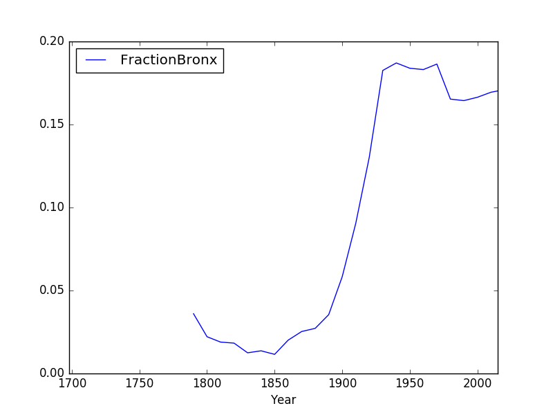
pop['Fraction'] = pop['Bronx']/pop['Total']
and then can use it to create a new graph:
pop.plot(x = 'Year', y = 'Fraction')
We can save it to a file, by storing the current figure (via “get
current figure” or
gcf() function
and then saving it:
fig = plt.gcf()
fig.savefig('fractionBX.png')
shown in the following plot:
Putting this altogether, we have a program:
#Libraries for plotting and data processing:
import matplotlib.pyplot as plt
import pandas as pd

#Open the CSV file and store in pop
pop = pd.read_csv('nycHistPop.csv',skiprows=5)

#Compute the fraction of the population in the Bronx, and save as new column:
pop['Fraction'] = pop['Bronx']/pop['Total']

#Create a plot of year versus fraction of pop. in Bronx (with labels):
pop.plot(x = 'Year', y = 'Fraction')

#Save to the file:  fractionBX.png
fig = plt.gcf()
fig.savefig('fractionBX.png)
How can you modify the program to let the user specify the borough to compute the fraction of the population? When you have the answer, see the Programming Problem List.
More on the Command Line Interface
You can write programs in the Unix shell scripting language. Often
called
_scripts_,
they are typically used for tying together input and output from
different programs.
Let’s look at a sample script (from elf lord’s tutorials on linux):
#!/bin/bash
echo "hello, $USER. I wish to list some files of yours"
echo "listing files in the current directory, $PWD"
ls  # list files
Looking at this script line-by-line:
-
#!/bin/bashIt’s standard to include as the first line of your scripts that specifies the program that’s running (this is often called the “shebang” line). There’s different variants of shell scripts. We’re using the default for Ubuntu (the type of Unix running on the lab laptops, called bash, so, we start our script by specifying that we want to use the bash shell to evaluate it.
-
The command
echois similar toprint()in Python. It writes a message to the terminal:echo "hello, $USER. I wish to list some files of yours" echo "listing files in the current directory, $PWD"$USERis a built-in variable that store the name of the current user. Similarly, the built-in variable, $PWD, stores the current directory (folder) that you are in. -
(NOTE: $USER might not print anything on gitbash installed on windows) Lastly, our scripts can include any of the Unix commands that you have already learned. The last line of this file lists the files in the current directory using the ls command:
ls # list filesIn the shell, the different types of quotes have similar, but different, meanings. We’ll use the double quotes since strings in double quotes will have special characters (like
\nfor newline) interpreted as in Python and C++.Use the 'nano' command to save the above script as "helloScript.sh" from your terminal: Type:
nano helloScript.shOnce the file is open copy the above script into the nano editor which opened up. , after you are done click 'cntrl+X' on your keyboard followed by 'Y' in order to save the changes of the file you created locallyNext, we’ll change the permissions on the file, so that we can run it directly, by just typing its name:
chmod +x helloScript.sh(changes the “mode” of the file helloScript to be executable– if you name it something else, replace the name in chmod command above).* To run your first shell script, you can now type its name at the terminal:
./helloScript.sh
What’s Next?
If you finish the lab early, now is a great time to get a head start on the programming problems due early next week. There’s instructors to help you, and you already have Python up and running. The Programming Problem List has problem descriptions, suggested reading, and due dates next to each problem.